


To enter a negative value into a Microsoft Excel sheet, precede the value with a hyphen character, (-), which represents the “negative sign.” Often though, you won’t want to display that character. Instead, you might want Excel to display negative values in red, or with parentheses, or both. Microsoft Excel provides two ways to do so: a format and a conditional format.
The first method is clean and quick because Excel offers four built-in formats for displaying negative values. The other method will do almost the same. You’ll use this feature when a format is already in use but doesn’t evaluate for negative values. To be honest, this won’t be an issue for most of us. However, it’s good to know that there is an alternative, if needed.
In this tutorial, I’ll show you both ways to display negative values in red in a Microsoft Excel sheet. I’m using Microsoft 365 desktop on a Windows 10 64-bit system, but you can use an earlier version. For your convenience, you can download the demonstration .xlsx and .xls files. If you’re using the .xls format, the Table object won’t be available, but you don’t need it. Excel for the web supports both methods.
SEE: Windows, Linux, and Mac commands everyone needs to know (free PDF) (TechRepublic)
Must-read Windows coverage
- CrowdStrike Outage Disrupts Microsoft Systems Worldwide
- 10 Best Project Management Software for Windows in 2024
- Windows 10 Extended Security Updates Promised for Small Businesses and Home Users
- Securing Windows Policy
How to use a format
Perhaps the traditional and easiest way to display negative values in red is to use an Excel format. Fortunately for this task, there’s a built-in format that automatically displays negative numbers in red.
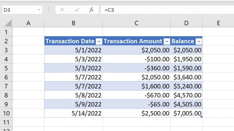
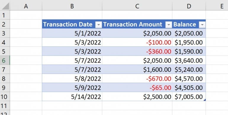
Our example data, shown in Figure A, is a simple transaction sheet, where the user enters debits as negative values. The name of this Table object is BalanceSheet. There’s a simple expression in column D that adds the previous balance to the current balance to return the balance after each transaction. If you’re following manually instead of using the demonstration file, enter the following into D3:
=C3
Then, enter the following into D4 and copy to the remaining cells:
=D3+C4
This is one of those times when a Table object throws in an unnecessary wrench because these two expressions aren’t the same: Excel will overwrite the expression in D3. If you’re using a Table and the second expression returns a value error, re-enter the expression, =C3, in D3. You can use a normal data range if you prefer.
Figure A
If you want debits displayed in red, apply an Excel format as follows:
- Select the currency values in C3:E10.
- On the Home tab, click the Number group’s dialog launcher. In Excel for the web, choose More Number Formats from the Number dropdown.
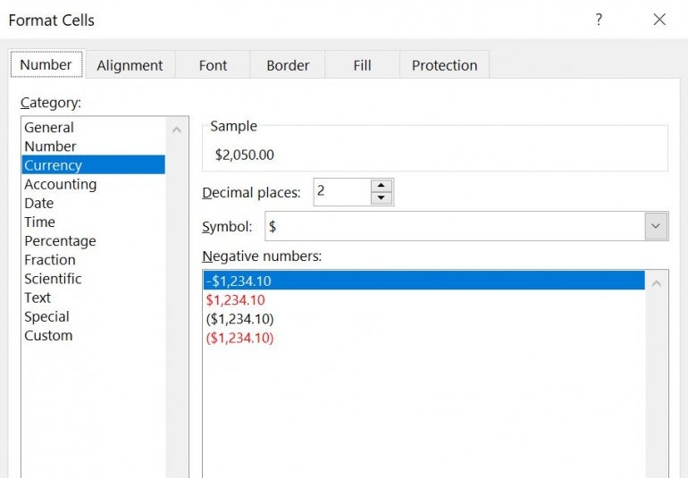
- In the resulting window, choose Currency from the Category list — if you’ve already assigned a Currency format, Excel will select Currency for you. Figure B shows the built-in Currency formats below the sample. There are four formats for negative numbers.
- Choose the last format, the one that displays the number in red and wrapped in parentheses.
Figure B
As you can see in Figure C, the format displays negative values—the debits—in red. In addition, Excel wraps them in parentheses. The user still enters the values as negatives by preceding the values with the hyphen character (-), but the format won’t display the hyphen.
Figure C
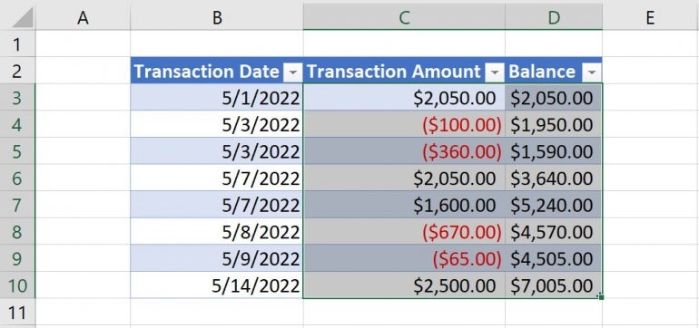
Although we applied the format to both columns, none of the values in column D are red. That’s because there are no negative values in that column. But, if one pops up, the format will apply.
If you’d rather not apply a format, or you’ve already applied a format that does something else, you can use conditional formatting.
How to use conditional formatting
A simple format won’t always be the answer. When this is the case, use conditional formatting. It’s almost as easy; it takes only a few more steps.
To apply a conditional format for only negative values, do the following:
- Select C3:D10.
- On the Home tab, click Conditional Formatting in the Styles group.
- From the dropdown, choose New Rule.
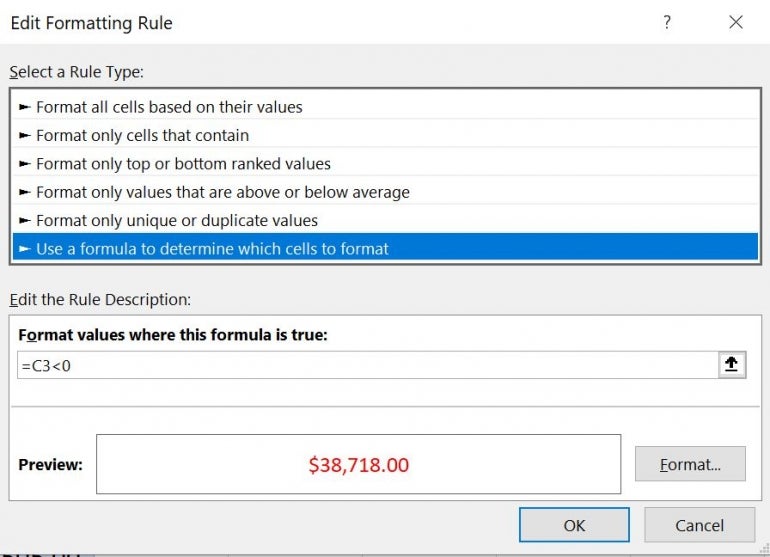
- In the resulting window, choose the Use a Formula to Determine Which Cells to Format option in the upper pane.
- Enter the simple expression, =C3<0 in the lower pane. When applying this to your own work, be sure to refer to the first cell in the selection. In our case, that’s C3.
- Click Format.
- Click the Font tab. You could click the Number tab, which allows you to set the same built-in format used in the first section. Remember though, we’re pretending that option isn’t available.
- From the Color dropdown, choose red.
- Click OK. Figure D shows the expression and the format.
- Click OK to return to the sheet.
Figure D
The conditional format will display the same values in red that the format does. However, as you can see in Figure E, it doesn’t wrap the values in parentheses. The rule is simple: If the current value is less than 0, meaning the current value is a negative number, the expression is True, and Excel applies the format (the red font).
Figure E
As mentioned, the built-in format should be your go-to method, but you can use a conditional format if necessary. It’s always great to have alternatives.