


In an ordinary sheet, descriptive header text often inflates the width of columns, pushing important data off screen. Moving from screen to screen is tedious and often, there’s nothing you can do about it. But, when the problem is the header text, you have choices. In this article, I’ll show you three cell formats that reduce the width of the header cells so you can get all of that data back on a single screen.
More about Software
- Software Installation Policy
- Five Methods to Insert a Checkmark Into Microsoft Office Products
- How to Hide and Handle Zero Values in an Excel Chart
- How to Use Section Breaks to Control Formatting in Word
I’m using Office 365’s desktop version of Excel on a Windows 10 64-bit system, but you can apply these formats in older versions. You can use your own data or download the demonstration .xlsx and .xls files.
SEE: System update policy template download (Tech Pro Research)
Shrink to fit
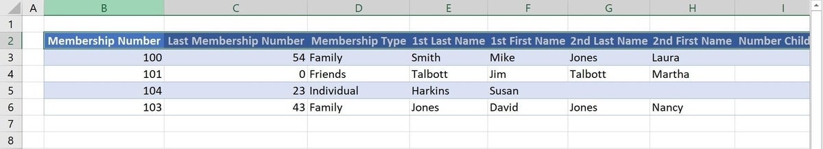
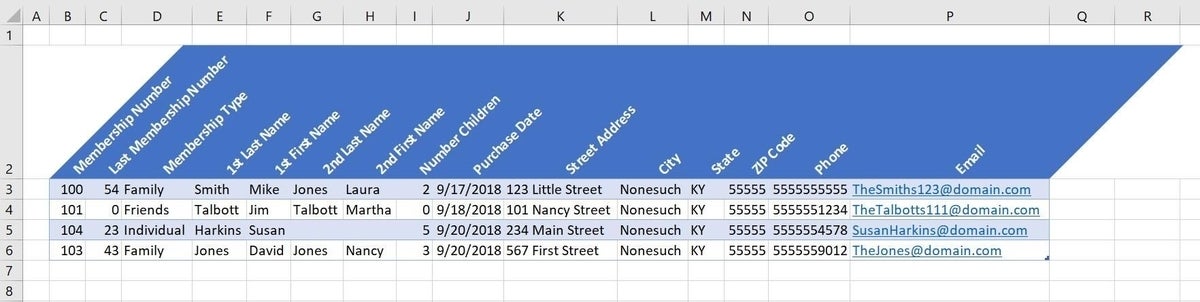
Figure A shows an example of what often happens when header text exceeds the actual data in the column. What you can’t see is that the data range extends to column P–you’re missing a lot. You could use a smaller font size, or you could delete some of the header text, but there are better choices. You might consider Shrink to fit, but I admit that it’s my least favorite of the three formats.
To apply this format, select the header cells, B2:P2, and click the Alignment dialog launcher (on the Home tab). On the Alignment tab, check the Shrink to fit option shown in Figure B. Or, press Ctrl+1.
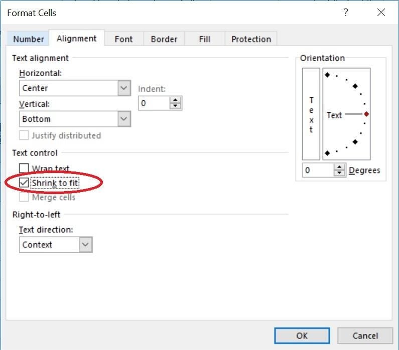
Figure C shows the results of reducing the width of column C–the effect is fairly dramatic. (You won’t see any difference until you reduce the width of the column.)
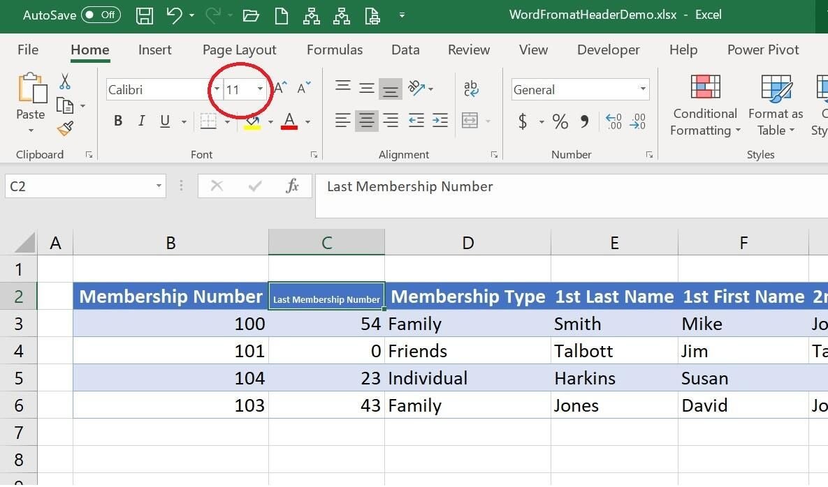
The text won’t increase if you increase the width of the column. In addition, the font size doesn’t actually change. If you check the Font Size control in the Font control, you’ll see that it’s the same as before. This format has limited use when fitting header text, but you should know it’s available.
Before continuing, be sure to remove the Shrink to fit format if you’re following along with the example because it’ll change the results of the next section, which introduces the Wrap Text format.
Wrap Text format
The Wrap Text format forces text to wrap to multiple lines within a single cell to accommodate the cell’s width. It’s easy to use, but this format sometimes yields unexpected results and requires a bit of tweaking.
Before applying the format, reduce the width of the column(s) to accommodate the text instead of the headers. Most of the header text will disappear. It’s temporary so don’t worry. Then, select the header cells, B2:P2, and click Wrap Text in the Alignment group on the Home tab.
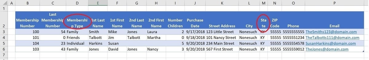
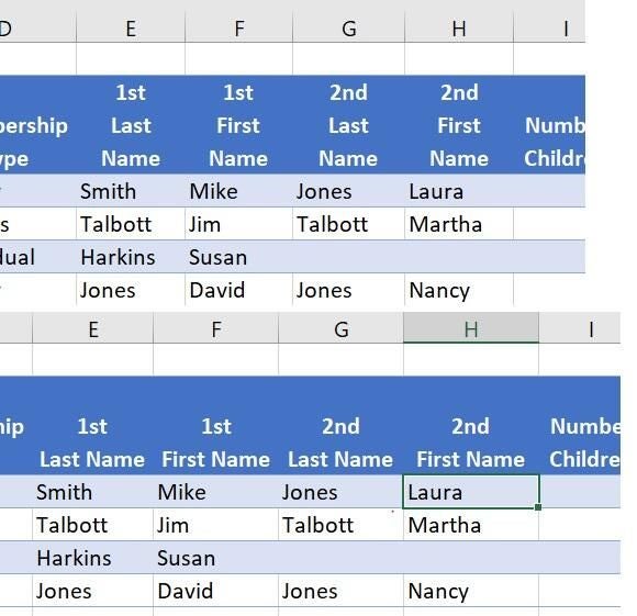
As you can see in Figure D, you usually have to tweak a column or two–or maybe even all of them. Specifically, columns D and M need to be a bit wider to keep the words Membership and State together. This format won’t keep words together automatically. However, we can see all of the data on one screen now.
Sometimes you’ll want to rearrange the words a bit. Columns E, F, G, and H illustrate this possibility. You might want Last Name and First Name to be on the same line. When this happens, force a “hard return” in the header text. To do so, select the cell and position the cursor before the word (in the Formula bar) you want to push to the next line and press Alt+Enter. If you end up with three lines of header text, as shown in Figure E, simply increase the width of the column(s) a bit.
Most of the time, Wrap Text gets the job done, but there’s one more format you can try. If you’re following along, remove the Wrap Text format from the header cells (it’s a toggle, simply select the cells and click Wrap Text) and then increase the column widths so you can see the full text headers.
Orientation
If Wrap Text isn’t appropriate, try the Orientation format, which rotates the font angle. Select the header cells, B2:P2, and click Orientation in the Alignment group on the Home tab. Figure F shows the result of choosing Angle Counterclockwise from the drop-down list. Many users press Ctrl+z to undo the change and give up because it doesn’t help and it looks odd. But the truth is, you’re almost there. (The online version doesn’t support the cell Orientation format.)
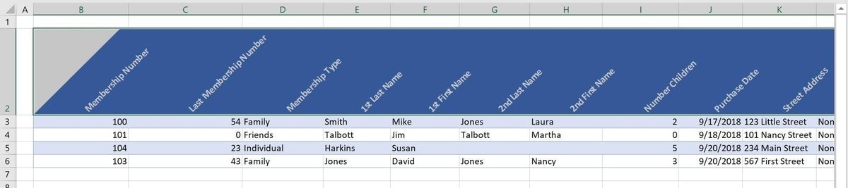
Similarly to the Wrap Text function, the column width is part of the show. Figure G shows the result of reducing the column widths to accommodate the data instead of the headers.
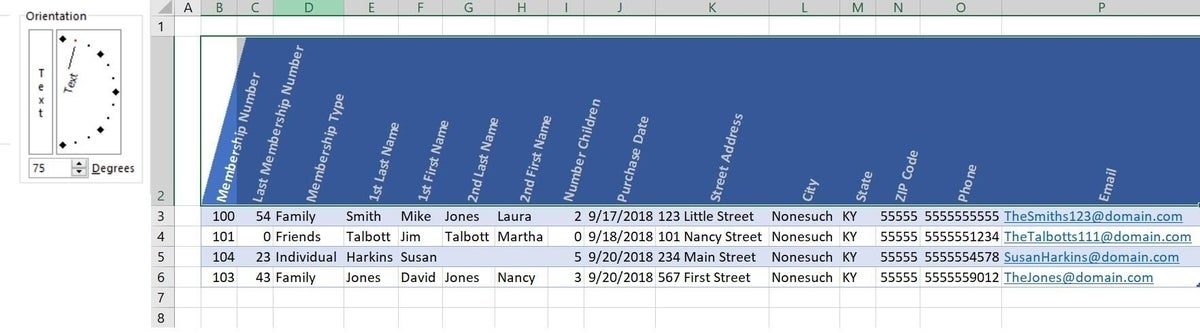
This feature has a number of settings, so if you don’t like this one, change it. Press Ctrl+1 and adjust the angle using the Orientation control to the right. You can drag the text line up or down or enter a number in the Degree control. By default, the degree 45 is represented in both spots. Figure H shows the result of dragging the Text line to 75. To quickly remove the format, enter 0 in the Degree control.
Send me your question about Office
I answer readers’ questions when I can, but there’s no guarantee. Don’t send files unless requested; initial requests for help that arrive with attached files will be deleted unread. You can send screenshots of your data to help clarify your question. When contacting me, be as specific as possible. For example, “Please troubleshoot my workbook and fix what’s wrong” probably won’t get a response, but “Can you tell me why this formula isn’t returning the expected results?” might. Please mention the app and version that you’re using. I’m not reimbursed by TechRepublic for my time or expertise when helping readers, nor do I ask for a fee from readers I help. You can contact me at susansalesharkins@gmail.com.
See also
- How to use Word mail-merge (TechRepublic)
- Office Q&A: How to use a macro to set Find defaults (TechRepublic)
- How to use Office Picture Layout options to quickly arrange pictures (TechRepublic)
- How to use Excel’s find feature to highlight or delete matching values (TechRepublic)
- Office Q&A: How to share Outlook 365 contacts (TechRepublic)
- Office Q&A: How to anchor image files in Microsoft Word (TechRepublic)
- Microsoft Office 365 for business: Everything you need to know (ZDNet)