
Excel can analyze mountains of data, but you might be working too hard if you’re not utilizing the Data Model feature to corral it. This feature lets you integrate data from multiple tables by creating relationships based on a common column. The model works behind the scenes and simplifies PivotTable objects and other reporting features. In this article, I’ll show you how to create a PivotTable using data from two tables by using the Data Model feature to create a relationship between the two tables before building the PivotTable.
I’m using Excel 2016 on a Windows 10 64-bit system. You can work with your own data or download the demonstration .xlsx file. The Data Model is available in versions 2013 and 2016. Excel 365’s browser edition supports PivotTable objects. However, you can’t implement the Data Model in the browser.
A simple problem
Now let’s suppose you’re working for a large grocery franchise and you want to analyze shelving data. You’ve imported a table of products and each product has a shelving code, which is, meaningless to you. So, you import a table of shelving codes that includes a helpful description, but how do you add the description with each record?
Most of us would use VLOOKUP() to add a column to the original data set. It’s what we know, and it works well unless you have thousands of records to analyze. But, even if it slows things down, it still works. Then, you’d most likely use a PivotTable to analyze the data set that now includes the description for each product. Thanks to Excel’s Data Model, you can bypass VLOOKUP() altogether and move straight on to the PivotTable.
Excel’s Data Model creates a relationship between two (or more) sets of data using a common field. In this case, the common field is Shelf Code, as shown in Figure A. We have two tables: the data table on the left and the lookup table on the right. Using Excel’s Data Model feature, we’ll display the description field instead of the shelf code when grouping and analyzing the values without using VLOOKUP() or any other functions. Displaying the description instead of the shelf code will improve the readability of the final product.
Figure A
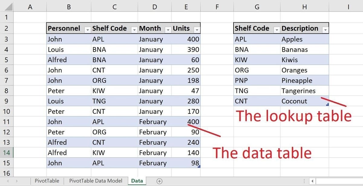
Two data sets related by the Shelf Code field.
If you’ve worked with databases, the term relationship is known to you. If you’re unfamiliar with the term, a relationship connects two sets of data by a common column (field) of values. By relating the two data sets, you can combine the data in meaningful ways.
SEE: Tap into the power of data validation in Excel (free PDF) (TechRepublic)
Convert the data to Table objects
You can’t create a relationship between ordinary data sets. The Data Model works only with Table objects. The example data sets have been converted already, but you might need to know how to do this. Fortunately, it’s easy:
- Click anywhere inside the data set.
- Press Ctrl+t or click the Insert tab and click Table in the Tables group.
- Check or uncheck the My table has headers options. In this case, it does (Figure B).
- Click OK.
- With the new Table still selected, enter a meaningful name in the Name Box control (to the left of the formula bar (Figure C). Be sure to press Enter. I named the original data set ProduceTable.
Figure B
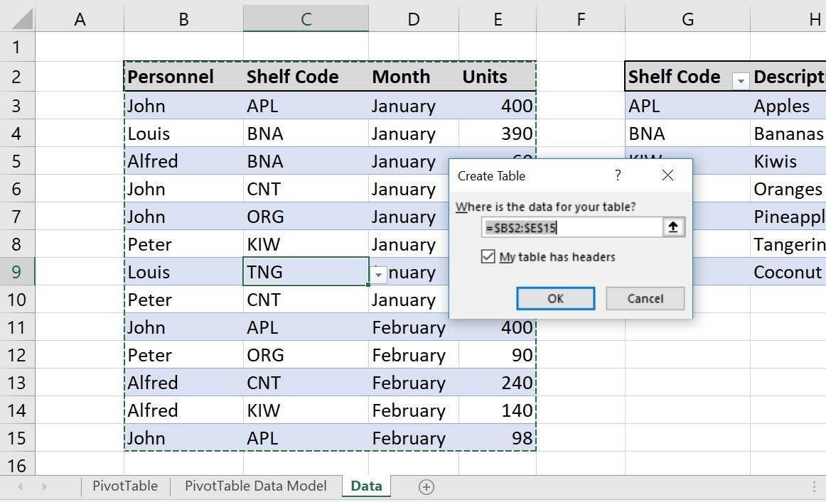
Convert the data set into a Table.
Figure C
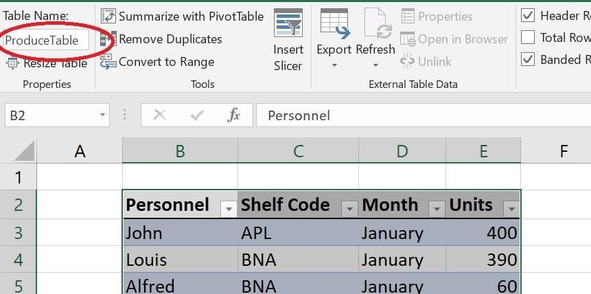
Name the Table objects so they’re easier to work with.
Repeat the process to convert the lookup values to a Table and name it ShelfCodesTable. With both data sets converted, you’re ready to create the relationship between them.
Create the relationship
Once both data sets are Table objects, you can create a relationship between them. To do so, click the Data tab and then click Relationships in the Data Tools group. Currently, there are no relationships, so the dialog will be empty. Click New to begin. In the resulting dialog, click the Table and Related Table dropdowns. You’ll find both Table objects listed, as shown in Figure D. (If you’re working with a file other than the demonstration file, you might see others listed.)
Figure D
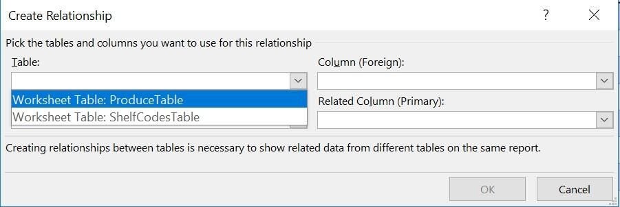
The Data Model can see both Table objects.
The Table contains the data you want to analyze in some way; the Related Table contains lookup values that will make the reported data more meaningful. It’s important to understand what’s going on, so let’s stop here to review. Our products table contains the data we want to analyze; it’s a list of product shelving information by personnel. All the values are repeated. Each person occurs multiple times, each fruit appears multiple times, even the months and shelf codes appear multiple times. The lookup table is the smaller table that contains unique rows. Each row contains a shelf code and a description. This table contains no repeated values. Each shelf code occurs only once in the lookup table, but it can occur multiple times in the produce data set.
The common column is the Shelf Code column; we’ll use both columns to relate the two Table objects. To create the relationship, choose ProduceTable from the Table dropdown and ShelfCodesTable from the Related Table dropdown.
Next, use the Column (Foreign) and Related Column (Primary) dropdowns to identify the columns that relate the Table objects–Shelf Code. Figure E shows the selected tables and columns.
Figure E
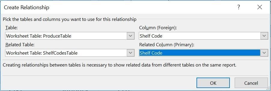
Set the tables and related columns in the relationship.
The column settings require a bit of explanation. Column (Foreign) defines the column in the produce table, where values can be duplicated. Related Column (Primary) defines the column in the lookup data set, where values are unique. The two columns will contain the same values. In a nutshell, we’re looking up a value in the lookup data set to display with the produce records.
Once you select all four settings, you’re ready to move on, so click OK and then Close. Excel creates the relationship behind the scenes, and it might take a few seconds. Excel combines the data, based on the Shelf Code field, in the Data Model, which contains the data and the relationships, but you won’t see it. What’s important to note at this point, is that the Data Model solution requires substantially less memory than a sheet full of expressions using the LOOKUP() function! Also, it will perform better in a large workbook. After creating the relationship, Excel will identify those tables as a Data Model Table, not a Worksheet Table in the dropdowns.
To see what Excel did, click Manage Data Model in the Data Tools group. If this option is greyed out, you don’t have a supporting version. Don’t worry–the benefits of the feature (known as Power Pivot) are still available, but you can’t view the combined tables. If it’s the first time you’ve used the feature, you might need to enable the Data Analysis add-in by clicking Enable when prompted.
Initially, the results are the same as the original data set, or ProduceTable. If you click Diagram View in the View group, you’ll see a diagram of the one-to-many relationship between the two Table objects, as shown in Figure F. Now you can create a PivotTable based on the new relationship. Close the Power Pivot window to continue.
Figure F
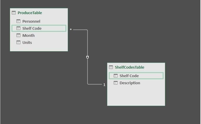
The asterisk identifies the many side; the 1 identifies the one side.
Create the PivotTable
Now you’re ready to create a PivotTable that evaluates both Table objects. Click the Insert tab and then click PivotTable in the Tables group. If you’re familiar with PivotTables, you might notice a new option: Use this workbook’s Data Model. You’ll only see this option when a workbook contains relationships. Select this option now, as shown in Figure G. Select the New Worksheet option, and then click OK to continue.
Figure G
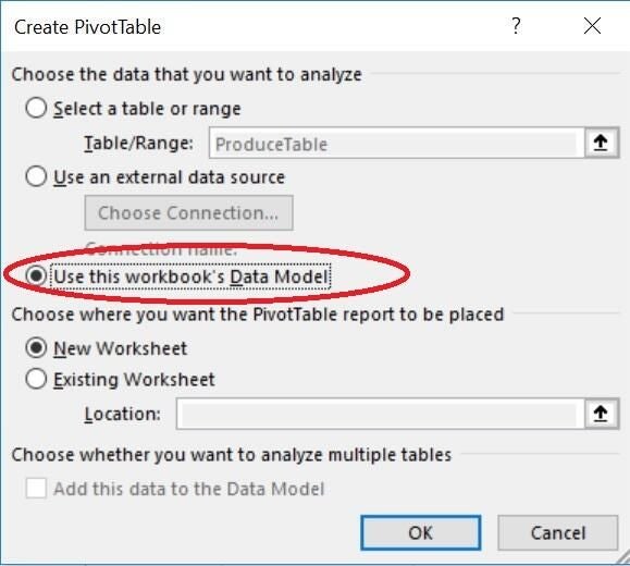
Use the Data Model to create a PivotTable.
The PivotTable Fields pane will display both Table objects. Notice the bold line at the top of the table icon? That means the table is part of a relationship, and hence in the Data Model. If that border is empty, the Table isn’t part of a relationship.
Now, lets create a PivotTable that counts the number of times each person shelved items (it’s a contrived example, but it’s simple and doesn’t add unnecessary steps). Expand the produce table and drag Personnel and Shelf Code to Rows, Month to Columns, and Shelf Code to Values, as shown in Figure H. (Excel will default to a count.) On the Design tab, I chose Light Blue, Pivot Style Light 9 to distinguish the data from the labels.
Figure H
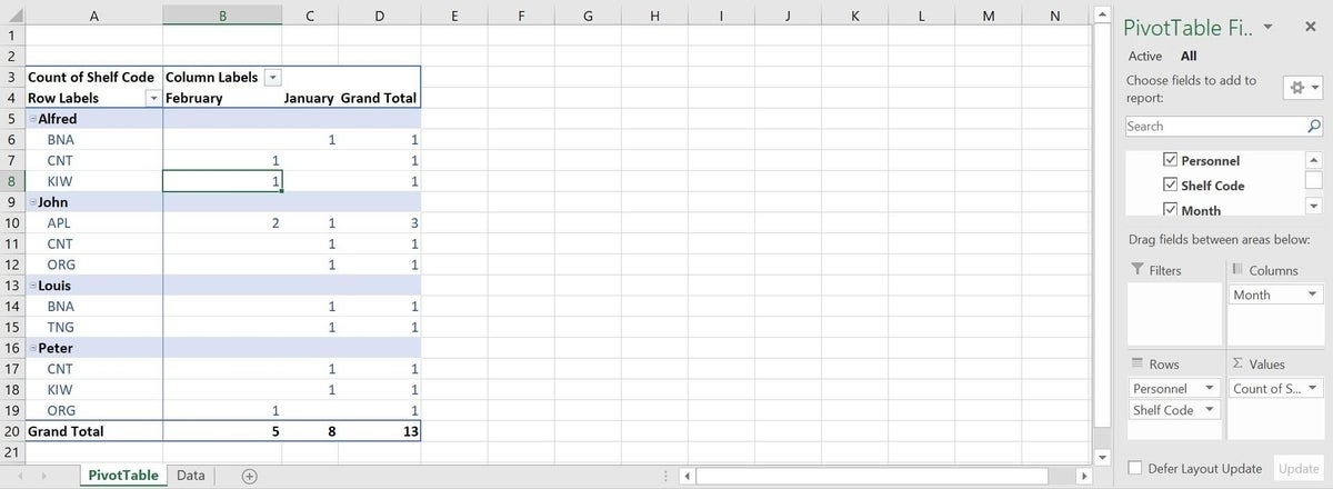
Create the simple PivotTable.
As you can see, those shelf codes are meaningless–to most of us anyway. Here’s where the Data Model magic comes into play. Remove the Shelf Code field from the Rows section. Then, expand ShelfCodesTable in the upper pane and drag the Description column to the Rows section. As you can see in Figure I, you now see meaningful descriptions that make sense!
Figure I
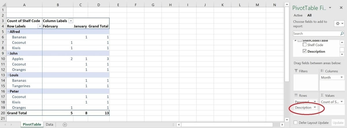
Display descriptive labels instead of meaningless codes.
Once you get the hang of it, you won’t need to replace columns as we just did. That tiny bit of drama was solely for effect!
Potential
At first, it seems like you’ve simply traded chores–creating a relationship instead of adding the VLOOKUP() function, but that’s because the example is simple. Once the relationship exists, you can use it in any number of ways. Trust me, once you apply it in the real-world situation, you will realize the value of having the relationship in place.
Send me your question about Office
I answer readers’ questions when I can, but there’s no guarantee. Don’t send files unless requested; initial requests for help that arrive with attached files will be deleted unread. You can send screenshots of your data to help clarify your question. When contacting me, be as specific as possible. For example, “Please troubleshoot my workbook and fix what’s wrong” probably won’t get a response, but “Can you tell me why this formula isn’t returning the expected results?” might. Please mention the app and version that you’re using. I’m not reimbursed by TechRepublic for my time or expertise when helping readers, nor do I ask for a fee from readers I help. You can contact me at susansalesharkins@gmail.com.
Also see:
- 5 ways to modify and customize styles in Microsoft Word (TechRepublic)
- How to use COUNTIFS() to compare multiple data sets (TechRepublic)
- Office Q&A: An easy Word Replace trick for a big problem and exposing duplicate records in Excel (TechRepublic)
- How to use Excel formulas to compare multi-column lists (TechRepublic)
- How to use Excel’s conditional formatting to compare lists (TechRepublic)
- Microsoft to add new geography, stocks data types to Excel (ZDNet)

