


Image: simpson33, Getty Images/iStockphoto
Must-read Windows coverage
- CrowdStrike Outage Disrupts Microsoft Systems Worldwide
- 10 Best Project Management Software for Windows in 2024
- Windows 10 Extended Security Updates Promised for Small Businesses and Home Users
- Securing Windows Policy
When entering data in Microsoft Excel, an autocomplete feature attempts to help. You probably use this feature a lot—it’s convenient, reduces data entry keystrokes, and helps avoid typos. It’s an on-the-fly feature of convenience. Wouldn’t it be great if you could use this autocompleting feature to search for data? Well, you can.
I’ll show you how to combine this behavior in Excel in a combo box with a VLOOKUP() function. The control will let you search by character using its autocomplete behavior, and the linked function will return a corresponding value for each match.
I’m using Office 365 (desktop) on a Windows 10 64-bit system. You can download the demonstration .xlsm file or work with your own data. Neither the browser version nor menu versions of Excel will support this technique.
How to do a basic search in Excel
We want to enter characters one at a time and see the first matching value and a corresponding value. Excel’s autocomplete feature works with data input. You can’t use it to search an existing column of values–you use the feature to enter a new value.
SEE: 17 tips for protecting Windows computers and Macs from ransomware (free PDF) (TechRepublic)
Fortunately, Excel’s ActiveX combo box control offers the same autocomplete behavior: As you enter characters, the control matches the first value in the populated list that matches the input characters. That’s an easy fix to the first half of the solution, but we still want to know more about the matching record.
For instance, let’s suppose you want to know the unit price for a specific category in the simple data set shown in Figure A. You know the category starts with the letter B, but you can’t remember the exact category name. (The example is contrived, but bear with me.) Using the combo box, matching categories to the letter B is easy. To get the unit price, we’ll link the combo box to a VLOOKUP() function. As you enter characters, the VLOOKUP() function will return the currently matched category’s unit price. For example, if you enter B, the combo will first match Baked Goods & Mixes and return the unit price of $2.50. If you then enter E (Be), the control returns Beverages and returns the unit price of $39.
Figure A
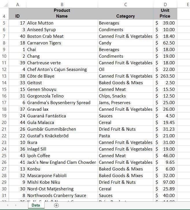
Looking at the actual data, you might expect B to return Beverages because that value occurs before Baked Goods & Mixes in the category column. Don’t worry about that discrepancy now–it’ll make sense in a bit. In a nutshell, the control’s list will be alphabetized even though the data isn’t. Now, let’s get started by adding a combo box.
How to add a combo box in Excel
The first step is to embed a combo box and populate it with a unique list of category values so we can take advantage of its autocomplete behavior. Before we add the combo box, let’s create a unique list of category values as follows:
- Select the data source, C4:C49.
- Click the Data tab and then click Advanced in the Sort & Filter group.
- In the resulting dialog, click the Copy To Another Location option. The List range should be correct because you selected it before you started.
- Enter F4 as the Copy To setting.
- Check the Unique Records Only option (Figure B) and click OK.
Figure B
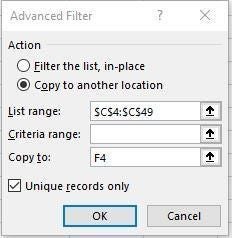
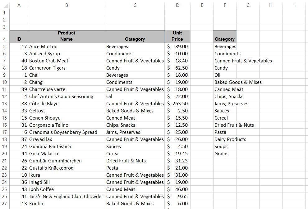
Figure C shows the unique list next to the original data source. In a working sheet, you should put this list in an out-of-the-way spot, but for our purposes, it’s convenient to see what’s going on. Before you continue, run a quick sort on the unique list of categories—if prompted to, do not expand the sort selection.
Figure C
With a unique alphabetized list available, let’s embed a combo box above the data set. (Insert a few rows about your data if necessary.) Click the Developer tab and then do the following:
- In the Controls group, click the Insert dropdown and then choose Combo Box from the ActiveX Controls section.
- Embed the control over C2 and resize as necessary.
- With the control selected, click Properties in the Controls group.
- Enter C1 as the LinkedCell setting and F5:F20 as the ListFillRange setting (Figure D). In a real sheet, you’d probably want to hide the linked cell under the control, but I want you to see the values change in real time.
- Close the property sheet.
- Click the Design Mode option in the Controls group to exit design mode.
Figure D
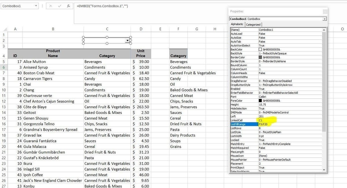
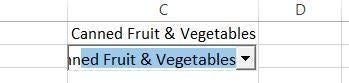
If you select the control and enter B, the control’s autocomplete behavior will return Baked Goods & Mixes. If you enter C, the control will return Candy. If you enter Cann, the control will return Canned Fruit & Vegetables, and so on. As you can see in Figure E, the linked cell, C1, also displays the matched results. Remember, the autocomplete feature is evaluating an alphabetized list, not the actual data in the Category column.
Figure E
We can use the control’s autocomplete behavior to match categories, but as yet we don’t know the matching category’s unit price—that’s next.
How to use the VLOOKUP() function
We can see that the combo box is linked to cell C1. Now we’re going to add a VLOOKUP() function that references C1, and the function will return the unit price for the updating value in the combo box. In D2, enter the following function:
=VLOOKUP($C$1,C5:D49,2,FALSE)
Before we go any further, let’s quickly review VLOOKUP(). This function uses the following syntax:
VLOOKUP(lookupvalue, tablearray, columnindex, [rangelookup])
where lookupvalue is the value you’re matching; in this case, that’s the value in C1; tablearray is the source data that contains lookupvalue and the corresponding value you want to return, columnindex indicates the column the returned value is in, and rangelookup determines whether you want the first closest value or an exact match.
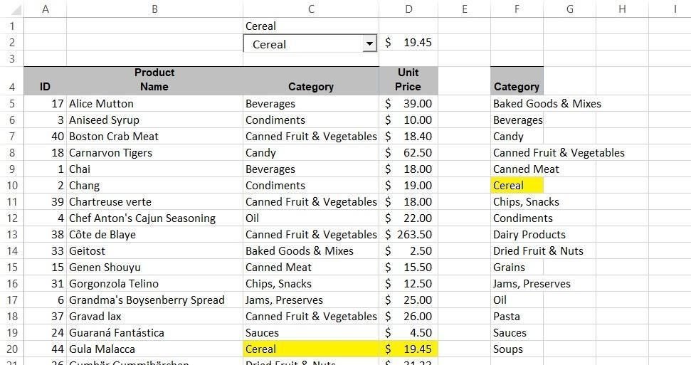
Let’s evaluate an example so this all comes together. Select the combo box. (If there’s no value selected in the combo box, the VLOOKUP() function returns #N/A—don’t worry about that right now.) Enter C and the combo matches Candy even though the first C value in the column is Condiments. Remember, the control’s list is alphabetized. The first Candy Unit Price value is $62.50, as shown in Figure F. Next, enter E (Ce) and everything updates to display the first Cereal value shown in Figure G ($19.45).
Figure F
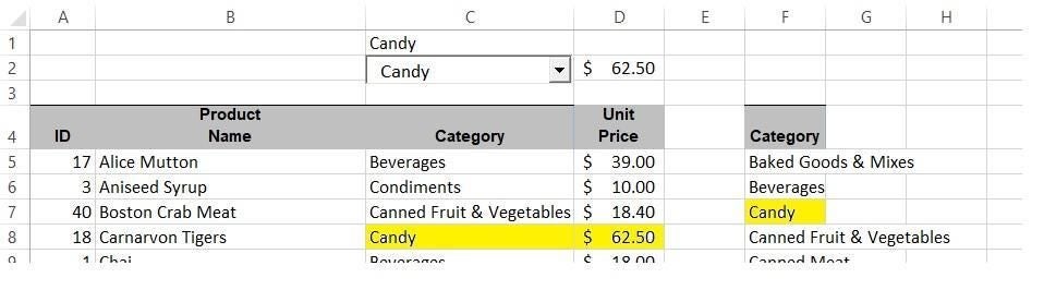
Figure G
I like this example because there are so many category values with the same first few characters.
How to use quick clear in Excel
As is, starting a new search is annoying because you have to clear the search string first. That’s too much work, so let’s add a small piece of code to do it for you.
First, save the workbook as a macro-enabled workbook (xlsm). Then, press Alt+F11 to open the Visual Basic Editor (VBE). Use the Project Explorer to select the appropriate sheet (that’s Sheet2 (Data) in the demonstration workbook). Enter the simple double-click procedure in Listing A.
Listing A
Private Sub ComboBox1_DblClick(ByVal Cancel As MSForms.ReturnBoolean)
‘Clear search combo.
Me.ComboBox1.Value = “”
End Sub
Don’t try to copy the code directly from this webpage–the VBE will complain about web characters that it can’t evaluate. Instead, enter it yourself or copy the code from this webpage first into Word or Notepad and then into the VBE.
The code is simple: Setting its value property to nothing clears the control’s text element, removing the previously selected value so you can quickly start again. This double-click trick isn’t intuitive, so if you share the file with other users, you’ll need to tell them about it.
How to inhibit the error in Excel
Right now, when the control’s text box is empty, the VLOOKUP() function returns an error. You can easily inhibit that display using the IFERROR() function as follows:
=IFERROR(VLOOKUP($C$1,C5:D49,2,FALSE),””)
When you clear the control, the results of the VLOOKUP() function will disappear, rather than display the error.
How to use easy search in Excel
This simple control and function combine to return a corresponding value from a data set. The function updates as you add characters. When you’re done, a double-click clears the search string.
While it’s convenient, it does have a limitation: It stops at the first matching value. There’s no way to browse for other matching values in the same column.
Stay tuned because over the next few months, we’ll create more complex search controls.
Send me your Microsoft Office questions
I answer readers’ questions when I can, but there’s no guarantee. Don’t send files unless requested; initial requests for help that arrive with attached files will be deleted unread. You can send screenshots of your data to help clarify your question. When contacting me, be as specific as possible. For example, “Please troubleshoot my workbook and fix what’s wrong” probably won’t get a response, but “Can you tell me why this formula isn’t returning the expected results?” might. Please mention the app and version that you’re using. I’m not reimbursed by TechRepublic for my time or expertise when helping readers, nor do I ask for a fee from readers I help. You can contact me at susansalesharkins@gmail.com.