How to count individual cells within a row by their fill color in Excel

The article How to easily sum values by a cell’s background color in Excel shows you an easy way to combine built-in features to count or sum values based on the fill colors. This technique requires no special knowledge, but it’s limited. You can’t use it to evaluate individual cells within a row; filtering is a columns-only feature. Furthermore, Excel offers no feature or function to directly evaluate cells by their fill color. In this article, I’ll show you how to do so. It’s not a clear-cut solution, and without a bit of inside knowledge, you’d most likely not figure it out on your own. The thing to remember is that we’re counting cells, not records.

SEE: Office 365: A guide for tech and business leaders (free PDF) (TechRepublic)

I’m using Microsoft 365 on a Windows 10 64-bit system, but you can use older versions. You can work with your own data or download the demonstration .xlsx file. (I’m including the menu version format, but it might not work reliably.) This solution isn’t appropriate for the browser edition. In addition, this technique works with fill colors applied directly or via styles; it won’t work with conditional formatting; that magic requires a Stephen Hawking level Hail-Mary pass.

This article is based on a question sent by Vic Micallef.

The data and the problem

If you’re a database person, you think in fields, or columns. Rows are important when you’re normalizing tables in a relational database, and then when reporting, but you analyze columns (mostly). Sheets are a bit different, and sometimes you need to evaluate values across columns in a single row. For the most part, Excel handles this situation fine. Unfortunately, there’s no built-in function or feature (to my knowledge) that makes it easy to evaluate cells by their fill color, across a row. Before you say it, no, reconstructing your data isn’t always a choice.

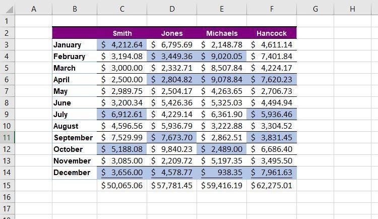
Now, let’s look at a simple sheet, Figure A, where random cells have a light blue fill color. For our purposes, it doesn’t matter what the color represents, but it is important to note that the color was applied directly (not conditionally). To count the number in a column, we could use filtering and the SUBTOTAL() function. Because we want to count filled cells across each row, we’ll have to work a bit harder (but at least it isn’t rocket science).

Figure A

If you search on this subject, you will find solutions that use GET.CELL to do the same thing that filtering does, but be careful. Those solutions don’t count individual cells within a row (or record). For instance, if you’re counting the fill color blue in our demonstration sheet, the count for row 3 is 1. We’re going to use GET.CELL to create a matrix. Then, we’ll use COUNTIF() to return the number of a specific fill color for each row.

This next step is very important; don’t skip it. If you’re using the .xlsx format, save the workbook as a macro-enabled file. 

How to implement GET.CELL

The CET.CELL is an old function that comes with limitations. Most importantly, you can’t directly reference it; in other words, you can’t enter =GET.CELL(38,C3) and return the color code for cell C3. Instead, you apply the function to a named range. Second, the way I’m using it allows only for counting adjacent cells within a row. If you insert a column between the data set and the matrix you’ll create later, the function still works, but it’s one column off. In addition, you can’t use it to count (individual) filled cells in a column. It’s a very specific solution.

Now, let’s put GET.CELL into play. Do the following to create a named ranged that can be used to return any cell’s fill color:

1. Click the Formulas tab, then click Define Name in the Defined Names group, and choose Define Name from the dropdown list.
2. In the resulting dialog, enter a name for the range, such as ColorCode.
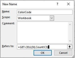
3. In the Refers To control, enter the following expression: =GET.CELL(38,Count!C3), where Count is the sheet name and C3 is the data set’s anchor cell. (See Figure B).
4. Click OK.

Figure B

At this point, nothing has changed visibly. It’s time to use the range ColorCode to return codes for filled cells.

How to use ColorCode

Right now, you don’t know the color code for any cell in our data set. To remedy that, we’ll create a small matrix, directly adjacent to the data set. (If you leave a blank column between the data set and the matrix, this solution will return erroneous results.)

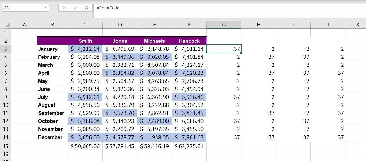
To create the matrix, enter the following expression in G3:

=ColorCode

which returns the value 37–that’s the fill color code for C3. Copy that expression to H3:J3. As you can see in Figure C, ColorCode returns the fill color for cells C3, D3, E3, and F3. This is possible because the reference you used when creating the range ColorCode, C3, is relative. If you made that reference absolute, $C$3, it would always return 37. Select G3:J3 and copy the four expressions to the remaining rows, completing the matrix shown in Figure D.

Figure C

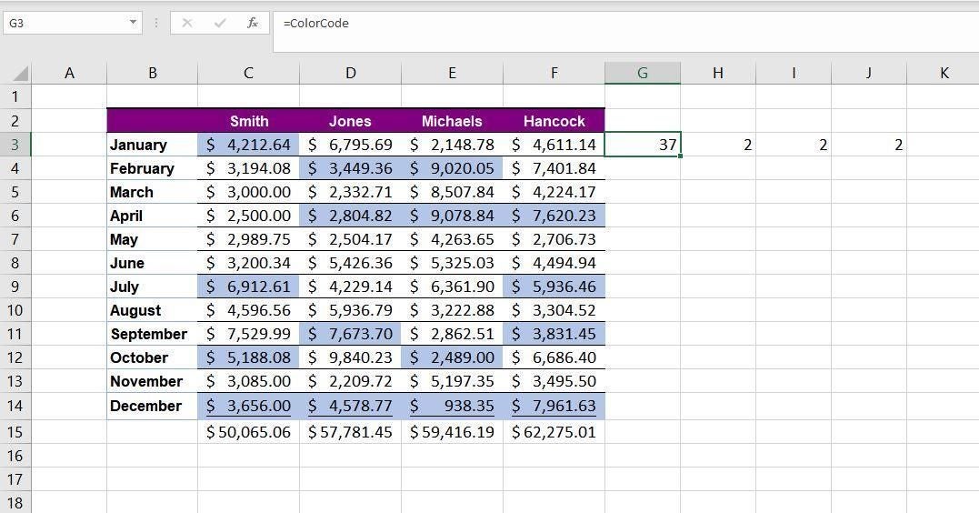
Figure D

The matrix isn’t dynamic; see the Limitations section below. We still don’t know the count of the blue filled cells in any row. We’ll tackle that next.

How to count the color codes

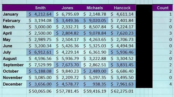
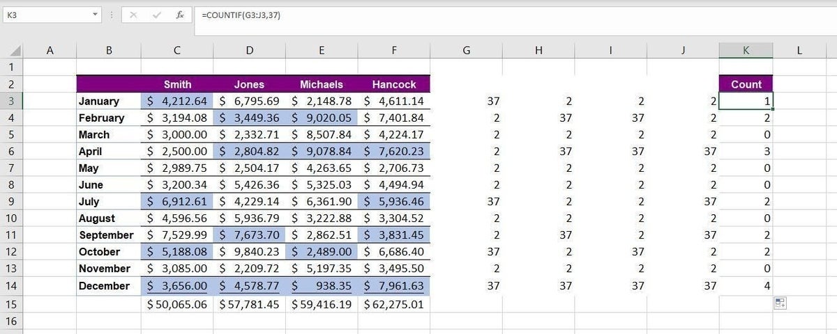
As is, the matrix returns the fill color codes for each cell in the data set. Using COUNTIF(), we can easily count the blue cells in each row. To accomplish this, enter =COUNTIF(G3:J3,37) in K3 and copy to K14. The values in column K, shown in Figure E, are a count of the number of blue filled cells in the corresponding row. Specifically, 37 identifies the blue filled cells and the function counts only those cells within the corresponding row. There’s only one cell in row 3 where the fill color is blue, 37. In row 2, there are two cells, and so on.

Figure E

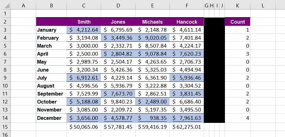
You’ll probably want to hide or otherwise obscure the matrix in G3:J3. I usually recommend that you not hide cells because they’re easy to forget, making the sheet harder to maintain. If you agree, reduce the width to the barest amount as shown in Figure F and apply back fill color.

Figure F

Variations

You can use GET.CELL to return a lot of information. The value we used, 38, returns a cell’s fill color. For instance, to sum the values, you’d use 5 instead of 38 when creating the range. Then, you’d use SUMIF() instead of COUNTIF(). A search on GET.CELL will turn up a list (Microsoft no longer maintains one that I could find.) You can also change the fill code being counted in the COUNTIF() function.

SEE: How to add a drop down list to an Excel cell (TechRepublic)

Limitations

As I mentioned, there are limitations–several. The matrix must be adjacent to the data set to work correctly. It won’t work for counting filled cells in columns. Because GET.CELL is no longer supported, it could stop working at any time. Modifications aren’t dynamic. If you change a fill color or update ColorCode, the matrix will not update automatically. In both cases, you must re-enter ColorCode, which is a nuisance. For that reason, I’m not convinced this is the most efficient solution; if you have a better idea, please share your thoughts in the comments section below.

Stay tuned

Because this solution is such a labor-hog, I’ll show you a macro in a follow-up article.