How to create a sorted unique list in an Excel spreadsheet

Lists are a fundamental part in almost any Microsoft Excel application, and fortunately, they’re easy to generate. There are two kinds of lists you might encounter: a static list and a list based on natural data. Without running a real poll, I suspect that the latter is the most common.

SEE: 30 Excel tips you need to know (TechRepublic Premium)

This type of list allows you to create dropdown lists and so on to aid data entry and protect the validity of your data. For instance, you might want to create a dropdown list that allows a user to choose employee or student names rather than typing them manually. This type of list is based on a data set that actually stores those values. In this article, I’ll show you two ways to generate a unique list of values based on a single column in a data set:

• An advanced filter
• UNIQUE()

I’m using Microsoft 365 on a Windows 10 64-bit system. UNIQUE() is available only in Microsoft 365, Excel for the Web, and Excel for Android tablets and phones. For your convenience, you can download the .xlsx demonstration file.

Pre-Microsoft 365: How to use the Advanced Filter in Excel

Once Excel introduced the AutoFilter feature, Excel’s original filtering features were often ignored. But occasionally, you’ll run into a situation that the AutoFilter can’t fulfill. When this happens, you can turn to Excel’s Advanced Filter feature, which supports more advanced options. This is where you turn when you need a unique list based on existing data. But before we get started, let’s review a few differences between the two filtering features:

• AutoFilter works with a static data set. Using the advanced feature, you can copy data to another location. You can remove duplicates from the source data set but doing so actually alters the data set.
• The advanced feature supports complex criteria.
• The advanced feature lets you extract a unique list or unique records—that’s what we’ll be doing.

Before UNIQUE() was available, you might have used an advanced filter to create a unique list of values. We’ll review this feature for those of you not using Microsoft 365. It’s important to remember that this technique isn’t dynamic, even if you use a Table object to store your data.

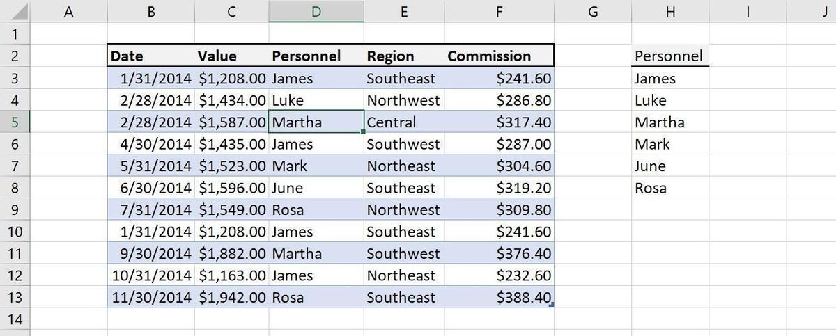
Figure A displays a simple data set with duplicate values in every column. Now, let’s suppose you need a list of unique values in the Personnel column.

Figure A

To create that list manually, do the following:

1. Click any cell in the data set.
2. Click the Data tab and then click Advanced in the Sort & Filter group.
3. Click the Copy to Another Location option.
4. Excel will display the cell reference for the entire data set or Table object as the List Range. If you retain this selection, Excel will return a unique data set based on all the columns. Instead, select the Personnel column by clicking the control and then selecting D2:D13. If you’re using a Table object, this feature might show the column name instead of the cell range.
5. Remove the Criteria Range if there is one.
6. Click the Copy To control and then select an out-of-the-way cell, such as H2. Be sure to specify a range that’s large enough so you don’t accidentally write over existing data.
7. Check the Unique Records Only option, as shown in Figure A.
8. Click OK.

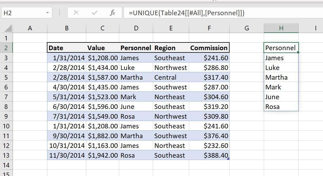
Figure B shows the unique list. There are six unique names in the Personnel column. The list is separate from your source data. In addition, the list isn’t dynamic. If you enter a record for a new employee, you must remember to update the list manually. If you want the list sorted, select the list, minus the header text and choose a sort order in the Sort & Filter group. Now let’s move on to the two functions that remove all of the manual steps and generates a dynamic list: UNIQUE() and SORT().

Figure B

How to use the UNIQUE() function in Excel

If you’re using Microsoft 365 or one of the 2019 standalone versions of Excel, you can quickly create a dynamic list using the UNIQUE() function. This function returns a list of unique values in a list or range, using the following syntax:

UNIQUE(array, [by_col], [exactly_once])

The array argument is the range you want to reduce to a unique list. The by_col argument is a Boolean value: TRUE compares columns and returns unique columns; FALSE is the default and will compare rows against rows and returns unique rows. The exactly_once argument is also a Boolean value: TRUE returns all distinct rows or columns that occur exactly once from the range or array; FALSE, the default, returns all distinct rows or columns from the range.

SEE: Windows 10: Lists of vocal commands for speech recognition and dictation (free PDF) (TechRepublic)

For our purpose of returning a unique list from a single column, we only need the array argument. Select a cell (I’m using H2 again) and enter the following function by selecting and not typing cells D2:D13, if you’re using a Table object—let Excel figure out the exact syntax. If you’re using a regular range, type the range address if you like. Figure C shows the results, which uses a spill range. When using UNIQUE(), you can display the header cell, or omit it by eliminating it from the selection.

Figure C

Microsoft 365 now supports what’s known as a spill range, which is the result of a dynamic array formula that returns multiple values—its output spills beyond the input cell. In short, a spill range is a range of calculated results from one formula. When you select any cell in a spill range, Excel highlights the entire range with a blue border and the function in the formula bar. You will always find the formula in the topmost cell.

Unlike the manual list we created earlier using an advanced filter, the results of UNIQUE() are dynamic. As you can see in Figure D, I added a new value to the Personnel column, and the list in column H updates automatically.

Figure D

How to use SORT() within the results of UNIQUE() in Excel

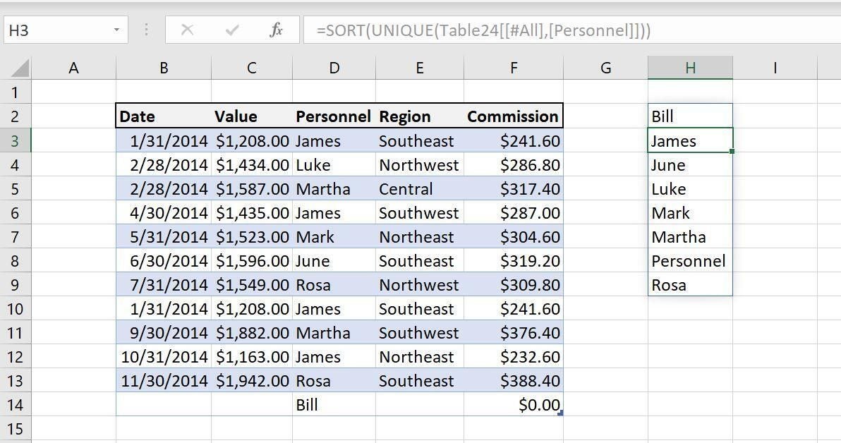
Unlike the resulting list generated by the advanced filter, you can use the SORT() function to sort the results of UNIQUE() and it couldn’t be easier. Figure E shows the result of wrapping UNIQUE() in SORT(). As you can see, the results are sorted, but can you find the error? The formula sorts Personnel with the rest of the values and you won’t want that to happen. The simple cure is to remove the header cell from the array range as follows:

=SORT(UNIQUE(D3:D13))

Figure E

If you’re still using an earlier version, use the Advanced Filter feature to create a static, unsorted list of unique values based on natural data. If you’re on Microsoft 365, wrap a UNIQUE() function in a SORT() function for a dynamic and sorted list.