
Image: PixieMe/Shutterstock
Filtering is a huge part of many Microsoft Excel sheets, and fortunately, there are many ways to do it. Microsoft 365’s new FILTER() function is a powerful upgrade. You won’t necessarily get different results using this new dynamic array function, but you’ll get those results using a single function! In this article, we’ll review the built-in Filter feature, then we’ll learn how to use the new FILTER() function.
I’m using Microsoft 365 (desktop) on a Windows 10 64-bit system. The built-in Filter feature is available in ribbon versions only. FILTER() is available to Microsoft 365, Excel 2021, Excel for the web, Excel for iPad and iPhone, Excel for Android tablets and phones. For your convenience, you can download the demonstration .xlsx file. This article assumes that you have basic Excel skills, but even a beginner should be able to follow the instructions to success.
SEE: 83 Excel tips every user should master (TechRepublic)
How to use the Filter feature in Microsoft Excel
Excel’s Filter feature lets you filter by multiple values, so you might not need the FILTER() function at all. For that reason, we’ll work through a quick example, so you can make an informed choice. Figure A shows a simple data set with filters. To apply filters, click the Data tab and then click Filter in the Sort & Filter group.
Figure A
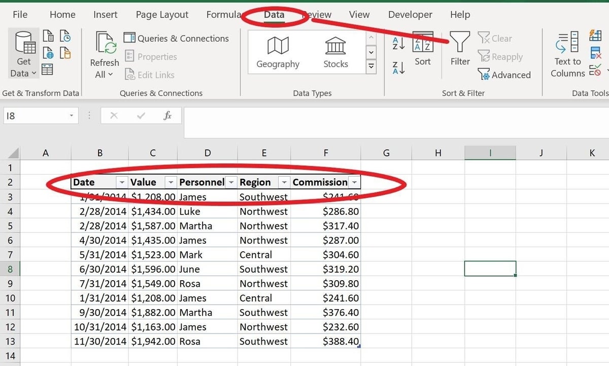
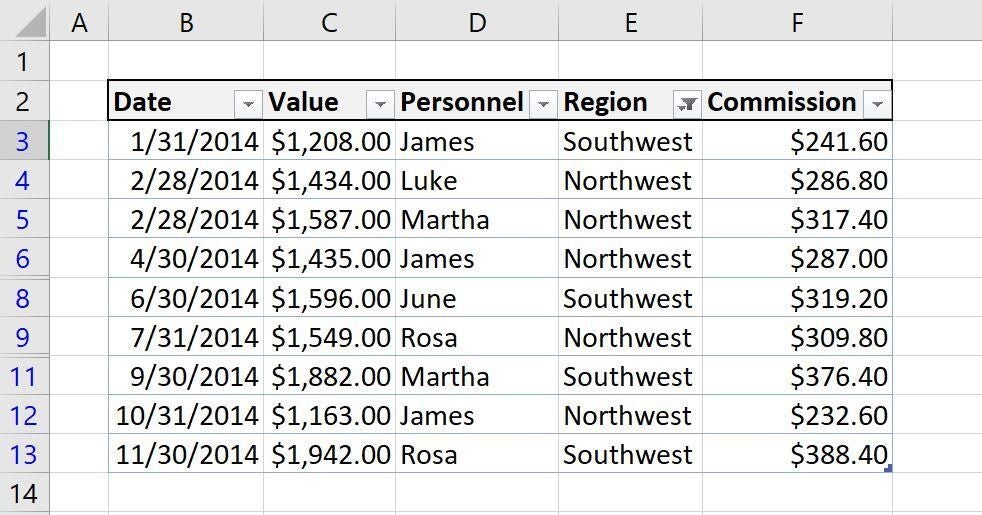
To use the filters, simply click the appropriate dropdown arrow in the header cell. Try that now by clicking the Region’s dropdown. The resulting pane lets you filter in many different ways. When no filter is set, all of the values are checked. To sort by one or more values, but not all of the values, uncheck the (Select All) item. Then, check the items you want to see. Figure B shows Northwest and Southwest selected. Subsequently, the filtered set shown in Figure C displays only records for those two values; there are no records for Central shown.
Figure B
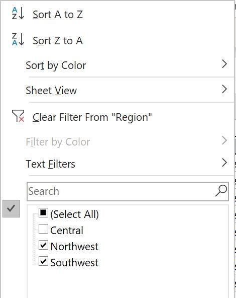
Figure C
This feature is flexible enough for most situations, but it has at least one limitation: You can’t display the filtered set in another location. This feature only filters the records in-place. Thanks to the new FILTER() function, doing so is almost as easy as using the Filter feature.
About the FILTER() function in Excel
Displaying a filtered set in another location makes for easy reporting and works especially well in a dashboard setup. Until FILTER() was introduced, getting a filtered set in another location required a bit of effort and skill.
FILTER() is one of Microsoft 365’s new dynamic array functions. It supports what’s known as a spill range, which is the result of a dynamic array formula that returns multiple values—its output spills beyond the input cell. In short, a spill range is a range of calculated results from one formula. When you select any cell in a spill range, Excel highlights the entire range with a blue border. You will always find the formula in the topmost cell of that range.
This function uses the syntax
FILTER(array, include, [if_empty])
where array identifies the source data, include identifies the value(s) you want to see in the filtered data set, and the optional if_empty specifies the value to display when the result is an empty set.
You can use FILTER() to return a single column or several. In addition, you can filter by a single column or several. Now, let’s put the FILTER() function to work.
How to use the FILTER() function in Excel
Using FILTER() has one requirement: You must use the same headers in the filtered set range. The original data set in B2:F14 is the source data. Simply copy the headers to another location.
Although not a requirement, the function is more flexible if you use input cells for the include argument. Figure D shows the necessary setup. We’ll use column I to create more flexible, dynamic, functions. The filtered data set will display in columns K through 0.
Figure D

Although you will seldom want to display the filtered results of only one column, it is possible, so let’s work through a quick example. Specifically, display the personnel for the Southwest region by entering the function
=FILTER(D3:D13,E3:E13=I5,”No results”)
into M3, as shown in Figure E. Then, enter Southwest into I5, the Region input cell. (Because the function is entered into a single cell and spills the results into the adjacent range, absolute referencing isn’t required.)
Figure E
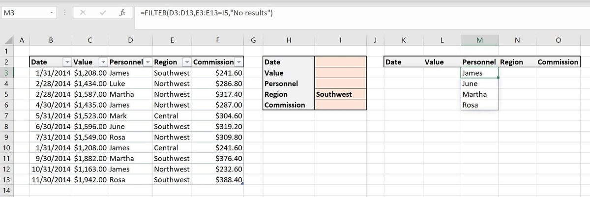
The result is easy to decipher by reviewing the function’s arguments:
- The array argument, D3:D13, displays only matching values from the Personnel column (column D).
- The include argument, E3:E13=I5, filters the list by the value in cell I5, which is Southwest.
The function returns only the personnel values for the Southwest region.
Let’s complicate things a bit by adding more display and filtering values. Enter the function
=FILTER(B3:F13,(D3:D13=I4)*(E3:E13=I5),”No Results”)
in K3, as shown in Figure F. (I’ve applied appropriate formatting because the FILTER() function can’t.)
Figure F

The include argument, (D3:D13=I4)*(E3:E13=I5), might be unfamiliar to you. The * character serves as an AND operator. In plain English, this argument filters by the personnel value in I4 and the region value in I5. The resulting filtered set contains only one record for James in the Southwest region. To apply an OR operator in the include argument, use the + character instead of the * character.
There’s one more way to improve results though. When the filtered set has multiple records, you might want to sort the results using SORT()
How to add the SORT() function in Excel
The SORT() function is another new dynamic array function. It returns a sorted array and uses the following syntax:
SORT(array,[sort_index],[sort_order],[by_col])
where array is the only required argument and identifies the range to sort. The optional arguments follow:
sort_index: A numeric offset value that identifies the row or column to sort by
sort_order: The number 1 for ascending sort or -1 for descending, with 1 being the default
by_col: The logical values TRUE for a row sort and FALSE for a column sort, with TRUE being the default
The current FILTER() returns only one record, so let’s remove James from I4 and return a descending sorted filtered set for the Southwest region, sorted by the Value column. To do so, enter the function
=SORT(FILTER(B3:F13,E3:E13=I5,”No Results”),2,-1)
in K3, as shown in Figure G.
Figure G

SORT()’s array argument is the entire FILTER() function. The sort_index value of 2 sorts by the Value column, the second column in array. The sort_index value is -1, which applies a descending sort. The result is a sorted filtered set that shows the highest value first for the Southwest region.
Worth noting
There are a few things you might want to include when applying FILTER() to your own work. First, the example sheet includes an input cell for each column in the source data set. However, I recommend that you include input cells only for the columns referenced by the FILTER() function’s include argument. Offering an input cell that doesn’t update the filtered set is confusing to users.
The built-in Filter feature converts the data set into a Table object. The FILTER() functions continue to reference the same source Table. When entering the functions, if you use the selection method to insert references, you will see Excel’s Table structure referencing at work instead of the actual range (array) references that I use. Don’t worry about it—everything will still work.
SEE: Windows 10: Lists of vocal commands for speech recognition and dictation (free PDF) (TechRepublic)
Because the source data is a Table object, everything is dynamic. If you add, delete or modify a record in the source data, the filtered data set will update accordingly.
In a true reporting or dashboard situation, consider using data validation to create dropdown lists for the input cells. Doing so will prevent errors when the input value is invalid.
You can wrap a FILTER() function in an aggregate function such as SUM(), AVERAGE(), and so on. Doing so will return only one value, the result of the aggregate on the filtered results of FILTER().
Stay tuned
Using FILTER() to match multiple values across multiple cells can be complicated. In fact, the built-in Filter feature is much easier to use in this respect. In a future article, I’ll tackle that requirement using FILTER(). We’ll continue the study with an article on filtering on value columns, such as Value and Commission.

