


Many organizations compare revenue and other assets from one year to the next to evaluate financial performance and refer to this as a year-over-year analysis. By measuring—comparing—revenue or some other asset, you can see if the organization is growing as intended. In this article, I’ll show you how to create a YOY chart by using Microsoft Excel’s PivotTable and PivotChart features.
SEE: Software Installation Policy (TechRepublic Premium)
Must-read Windows coverage
- CrowdStrike Outage Disrupts Microsoft Systems Worldwide
- 10 Best Project Management Software for Windows in 2024
- Windows 10 Extended Security Updates Promised for Small Businesses and Home Users
- Securing Windows Policy
I’m using Microsoft 365 on a Windows 10 64-bit system, but you can use an earlier version. I recommend that you hold off on upgrading to Windows 11 until all the kinks are worked out. For your convenience, you can download the demonstration .xlsx file. This feature isn’t supported by the older .xls format. Excel for the web supports both PivotTables and PivotCharts in an existing .xlsx file. You can also create a PivotTable in Excel for the web, but you can’t group columns. Nor can you insert a PivotChart.
What’s a year-over-year chart?
Most organizations rely on YOY charting to see if they’re growing at a rate that meets their goals. You don’t have to compare revenue. For instance, a call center might compare the increase or decrease in service calls over the last few years. In addition, an organization seeking investors or trying to sell the company will need to present favorable YOY analysis. It’s an effective way to evaluate performance.
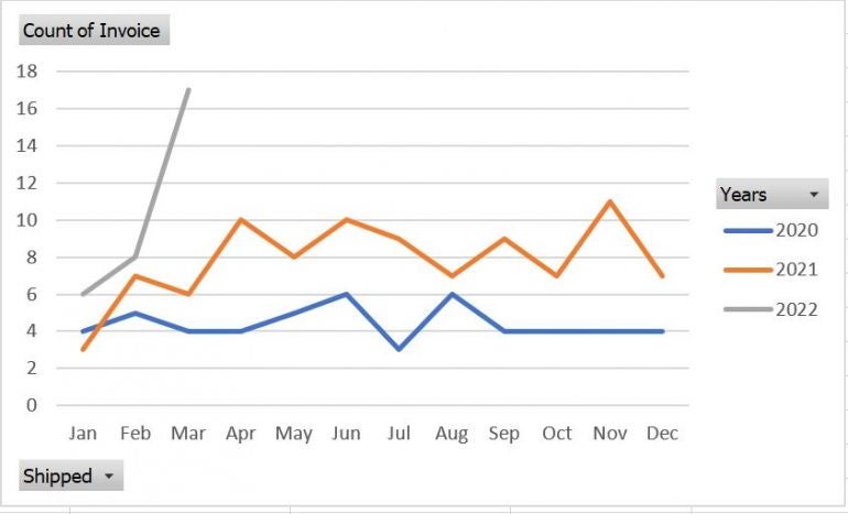
The YOY chart shown in Figure A displays a line for each year in the data set. If you want to compare the first quarter of 2022 to 2021 and 2022, you’d want to see three lines—one for each year, as shown in Figure A. What the data points represent depends on your needs. In this case, the chart compares the number of invoices each month.
Figure A
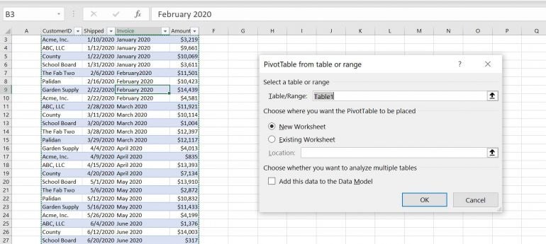
These comparisons can be fairly easy or very complex depending on the how the business stores its data. I recommend starting with a simple database type list if you can, and if you’re using Excel to analyze that data. For instance, the sheet in Figure B stores customer invoice information. Each record identifies the customer, the shipping date, the invoice month and the invoice total. (You can only see a few records for 2022, but the Table contains dozens of records for 2020, 2021 and 2022.)
Figure B

At this point, you know what a simple YOY PivotChart looks like and its purpose, and you’ve had a look at the source data. Let’s move on and build a PivotTable to support the PivotChart (Figure A).
How to build the PivotTable in Excel
Thanks to the data structure, the PivotTable will be simple to build. But before we do anything, let’s review what we want. For this example, we want to count the number of invoices by year and month. That means we need to group the records by months and years. If it sounds complicated, don’t worry, it isn’t.
Let’s continue by creating the PivotTable as follows:
- Click anywhere inside the Table data set.
- Click the Insert tab and choose PivotTable in the Tables group.
- Excel does a good job of determining your needs, as you can see in Figure C. Take a moment to review the settings and then click Insert.
Figure C
- In a new sheet, you’ll see an empty PivotTable frame and the Field list.
- Using Figure D as a guide, drag fields from the list to the appropriate list controls at the bottom. (You don’t need the CustomerID in the PivotTable.)
Figure D
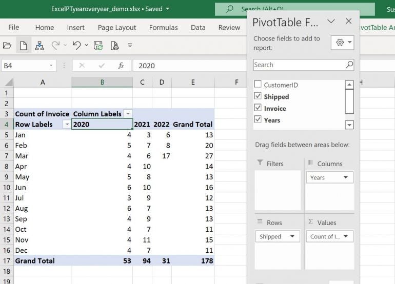
Are you wondering where the Years field came from? Excel automatically adds it when the source data includes a date field.
If your PivotTable doesn’t look the same, right-click any of the month cells (the first field to the left) and choose Group. In the By list, make sure Months and Years are selected, as shown in Figure E. It’s possible that you might have to unselect Quarters or Days.
Figure E

With the PivotTable data counting invoices by month and year, it’s time to create the PivotChart (Figure A).
How to create the PivotChart in Excel
At this point, you have a PivotTable that counts the number of invoices per month and by the year. From here, creating the year-over-year PivotChart is easy:
- Click anywhere inside the PivotTable you just created.
- Click the Insert tab and choose PivotChart from the Charts group.
- In the resulting dialog, choose Line in the list to the left, and click OK.
- Figure F shows the two pivot objects side by side.
Figure F
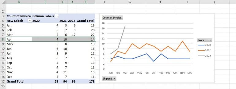
That was easy! Because the PivotTable does the grouping work, the PivotChart needs almost no input from you. The PivotTable tells a story that the data nor the PivotTable can tell. It looks like the first quarter of 2022 is off the charts, as they say. Of course, the number of invoices doesn’t reflect actual income. For that, you’d need to change the PivotTable.
How to sum invoice amounts in Excel
The YOY PivotChart might be helpful to someone on your team, but most everyone will be interested in revenue. To compare revenue over the three years we need to add the Amount field to the PivotTable. To do so, right-click anywhere in the PivotTable and choose Refresh from the resulting submenu. Doing so will add Amount from the data source to the field list.
Drag Amount from the field list to the Values control list and then delete the Count of Invoice field, as shown in Figure G.
Figure G
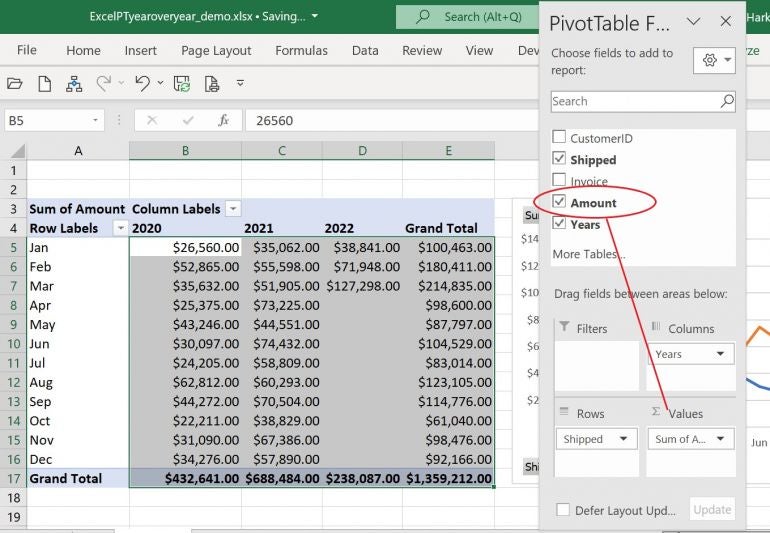
To delete it, click the dropdown and choose Remove Field from the resulting submenu. Figure H shows the updated PivotChart. 2022 is starting off to be a great year! Specifically, March 2022 was an amazing month.
Figure H
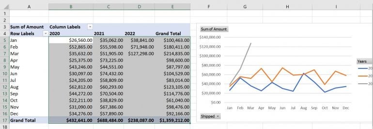
This type of chart provides a lot of information, and thanks to Excel’s two pivot objects, you won’t have to jump through hoops to produce it.