Image: Rawpixel Ltd, Getty Images/iStockphoto
Must-read Windows coverage
- CrowdStrike Outage Disrupts Microsoft Systems Worldwide
- 10 Best Project Management Software for Windows in 2024
- Windows 10 Extended Security Updates Promised for Small Businesses and Home Users
- Securing Windows Policy
Working with dates and times is a common need in an Excel sheet. If you’re lucky, the structure supports the way you use the sheet. Sometimes we inherit a sheet, or we have to accommodate a new request. In a nutshell, a date serial value can contain the date and time or only the date or time. Eventually, you might need to know how to extract the date and time from a serial value that combines both. In this article, I’ll show you a simple function, TRUNC() that can do both.
SEE: 69 Excel tips every user should master (TechRepublic)
I’m using Microsoft 365 on a Windows 10 64-bit system, but you can use earlier versions. You can work with your own data or download the demonstration .xlsx and .xls files. The browser edition supports the expressions in this article.
About date arithmetic in Excel
Unless you’re new to Excel, you’re probably a bit familiar with the way Excel stores dates and times using serial values. This section is a short review.
Dates usually look as you expect; for example, April 6, 2021, or 4/6/2021. There are other date formats that you’ll also recognize. Using specific date and time formats, you can display a date or time in many ways. That’s not how Excel stores a date, though—not as the formatted string that you see. Rather, Excel stores the value as a serial value where January 1, 1900, has a date serial value of 1 and adds 1 for every day moving forward in time. If you were to do the math, you’d find that the date serial value for April 6, 2021, is 44292.
SEE: Windows 10: Lists of vocal commands for speech recognition and dictation (free PDF) (TechRepublic)
To see this for yourself, enter the date April 6, 2021. Excel will display it as shown in Figure A because that’s the default date format. Don’t worry if you see something a bit different because you might be working with a different default (if someone changed it). To the right is the same date entered the same way, but the format is different; I changed it to General so you can the stored serial value. When you enter a date string, Excel formats it as a date using the date format, d-mmm-yy.
Figure A

The date is an integer; time is a decimal value. A day equals 24 hours. Twelve hours is half a day, or 0.50. For a comprehensive breakdown, see Table A. In the following sections, you’ll be working with complete serial values—dates that include both a date and time.
Table A
|
Format h:mm:ss |
Time Serial |
Time Equivalent |
|
23:59:59 |
0.999988426 |
23 hours, 59 minutes, and 59 seconds |
|
1:00:00 |
0.041666667 |
1 hour |
|
23:00:00 |
0.958333333 |
23 hours |
|
0:01:00 |
0.000694444 |
1 minute |
|
0:59:00 |
0.040972222 |
1 minute and 59 seconds |
|
0:00:01 |
1.15741E-05 |
1 second |
|
0:00:59 |
0.00068287 |
59 seconds |
How to extract the date in Excel
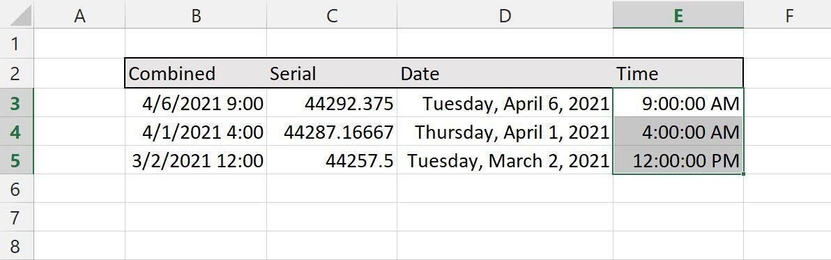
You’ll often work with date values that have no decimal value or time values. When the two are combined into one value, such as 44292.0412, they can be difficult to work with. For example, 44292.0412, 44292.0413, and 44292.000695 aren’t the same value, even though they share the same date. Figure B shows three combined serial values. Again, I entered the dates as literal date strings in the first column. To expose the serial values, I applied the General format to column C.
Figure B
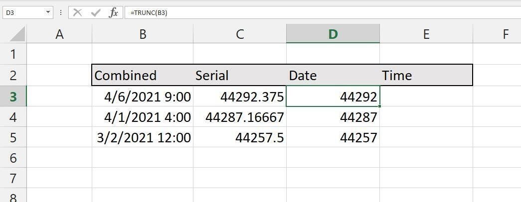
Column D contains the simple function
=TRUNC(B3)
copied to the remaining cells. As you can see, Excel applies the General format automatically and returns only the integer portion of the combined serial value in column B. You might be wondering why I didn’t use INT(). You can, but TRUNC() returns only the integer digits; INT() rounds a number down to the nearest integer. Because we’re working with positive dates values, it won’t matter, but negative dates are possible, so TRUNC() is the safer route.
How to extract the time in Excel
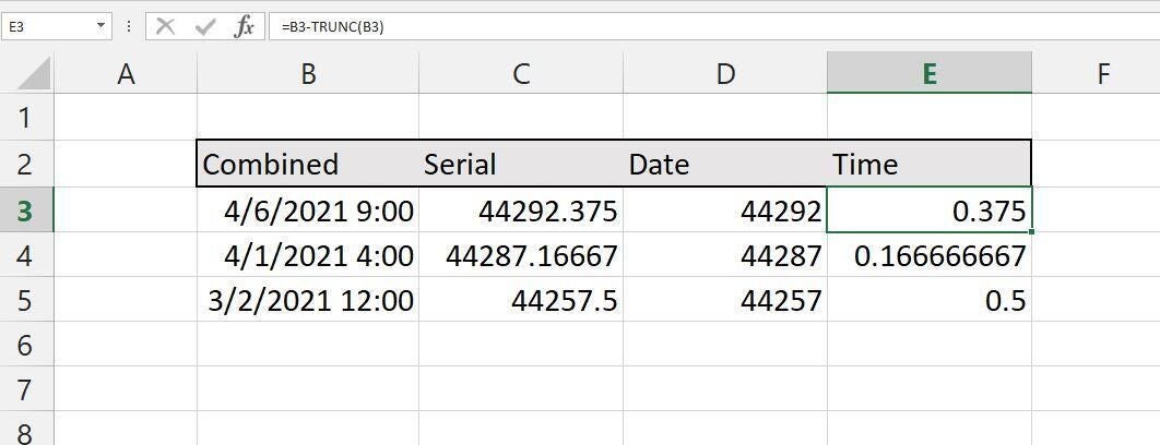
Dealing with time is often more difficult than dealing with dates. However, in this case, it’s nearly as simple using the TRUNC() function. Figure C shows the result of using the simple expression
=B3-TRUNC(B3)
and copying it to the remaining cells. In a nutshell, this expression subtracts the integer portion (the date) from the combined serial value. For example, the expression in E3 evaluates as follows:
=B3-TRUNC(B3)
=44292.375-TRUNC(44292.375)
=44292.375-44292
.375
Figure C
MOD() can be used, but TRUNC() evaluates only the exact components: the integer and the decimal. At this point, you can see the serial values that represent the date and time, but you don’t see the actual date and time strings that make sense to you.
How to add the formatting
The serial values don’t make sense to the viewer, so let’s format columns C and D, so they display something meaningful. First, select D3:D5, right-click the selection and choose Format Cells from the resulting submenu. In the resulting dialog, choose Date from the Category list. (You could also use the Format dropdown in the Number group.) The Type preview will update accordingly with examples. Choose the format that suits your needs, such as Wednesday, March 14, 2021, as shown in Figure D. Next, select E3:E5, right-click, choose Format Cells and choose Time from the Category list. Choose 1:30:55 PM from the Type list.
Figure D
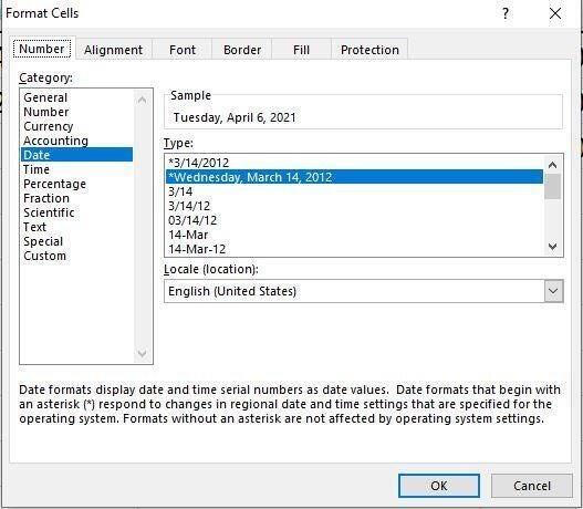
Figure E shows the results of formatting both columns of extracted serial values. The formatted values match perfectly to the combined serial values. We didn’t lose or add a thing. All we did was extract the integer and decimal values from the serial values in column B
Figure E