


Image: iStock/Rawpixel
Must-read Windows coverage
- CrowdStrike Outage Disrupts Microsoft Systems Worldwide
- 10 Best Project Management Software for Windows in 2024
- Windows 10 Extended Security Updates Promised for Small Businesses and Home Users
- Securing Windows Policy
Excel’s MINIFS() and MAXIFS() functions identify the lowest and highest values within a range, respectively, depending on one or more conditions. If the condition happens to have conditions of its own, these functions take on a new level of difficulty. In this article, I’ll show you two conditional format rules that highlight the minimum and maximum number within a range of years. We’re not looking for a single year as the condition! Rather, it can be any number of years inclusive on the first and last years in the range.
SEE: 60 Excel tips every user should master (TechRepublic)
I’m using Microsoft 365 on a Windows 10 64-bit system, but you can use earlier versions. The browser edition will support these functions. For your convenience, you can download the .xlsx demonstration file.
About MINIFS() and MAXIFS()
These two functions are super easy to use, taking the simple form
MINIFS(minrange,criteriarange1,criteria1[,criteriarange2,criteria2],…)
MAXIFS(maxrange,criteriarange1,criteria1[,criteriarange2,criteria2],…)
In a nutshell, these functions return either the minimum or maximum value within a range where criteria returns true. When a function has multiple criteria arguments, all must return true. Both functions work with values and dates, and the values don’t need to be sorted beforehand.
SEE: How to highlight unique values in Excel (TechRepublic)
The criteria
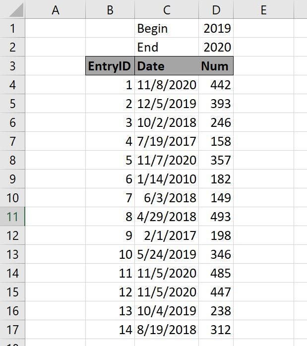
Now let’s look at the data we want to evaluate in Figure A. The dates in column D are from five years. Even without functions it’s easy to discern that 2020 is the most recent year, and 2010 is the least recent. We want to highlight the minimum and maximum value in column D within a period of years (the criteria).
Figure A
If you follow my articles, you know that I like to break things down into helper functions. You don’t have to use them but doing so is easy and it helps visualize how everything works together. Our first step is to create input cells for the first and last years in the year range: These are in D1:D2. The criteria, or condition, will include all the years inclusive of both years. Because there’s so much going on, we’ll break things down into simpler expressions and then combine them to create the conditional format rules.
SEE: How to use shortcuts to sort in Microsoft Excel (TechRepublic)
The expressions
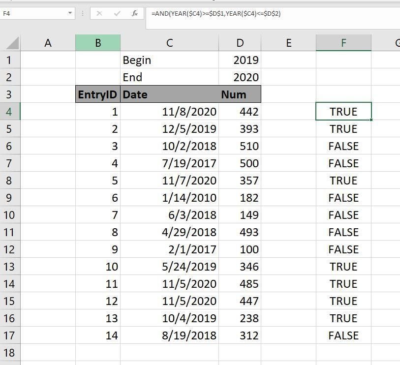
The first expression returns TRUE or FALSE. When TRUE, the corresponding date in column C falls within the conditional period of years; FALSE means the date doesn’t. We’re using an AND operator that uses equality operators to determine whether each year fits the condition or not.
Enter the first expression
=AND(YEAR($C4)>=$D$1,YEAR($C4)<=$D$2)
into F4 and copy to F17. Pay close attention to the relative and absolute references—they matter. If the year in column C is equal to or greater than the Begin date in D1 and that same year is equal to or less than the End date in D2, this function returns TRUE and FALSE if not. In Figure B, you can see that there are seven years in 2019 or 2020.
Figure B
We now know which dates fulfill the year period criteria—the TRUE values in column F tell us that. Next we need to know which value in column D is the highest or lowest, but only evaluating the values when the corresponding values in column F are TRUE.
SEE: 3 ways to suppress zero in Excel (TechRepublic)
The next two expressions, shown in Figure C, return the highest and lowest values inclusive of the two dates, respectively:
=MAXIFS($D$4:$D$17,$F$4:$F$17,TRUE)
=MINIFS($D$4:$D$17,$F$4:$F$17,TRUE)
Figure C
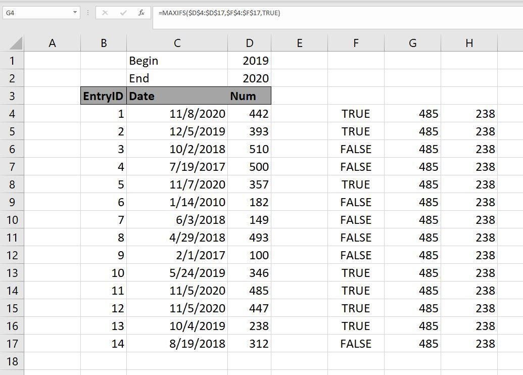
The criteria range is the AND operator expression in column F; the criteria is the TRUE value. In a nutshell, the MAXIFS() and MINIFS() functions evaluate only those values in column D where the value in column F is TRUE.
At this point, you have the conditional rules:
=$D4=MAXIFS($D$4:$D$17,$F$4:$F$17,TRUE)
=$D4=MINIFS($D$4:$D$17,$F$4:$F$17,TRUE)
You could hide column F, or not. You no longer need the functions in columns G and H—we just worked through those so you could visually work through the logic. Leave them for now so you can watch them update in the next section.
SEE: How to easily include dynamic dates in a Word doc using Excel (TechRepublic)
The conditional rule
Now that we have our two formulaic rules, let’s enter them and see how they work. To get started, select B4:D17 and then do the following:
- On the Home tab, click Conditional Formatting in the Styles group.
- Choose New Rule from the dropdown.
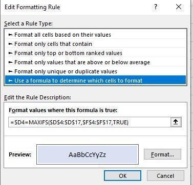
- In the resulting dialog, select the last option, Use a Formula to…, in the top pane
- In the lower pane, enter the expression:
=$D4=MAXIFS($D$4:$D$17,$F$4:$F$17,TRUE) - Click Format, choose a light blue fill color, and click OK.
- Figure D shows the expression and the fill format. Click OK.
Figure D
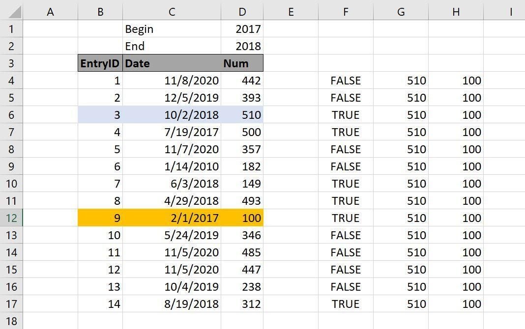
As you can see in Figure E, the record with the largest value in column D that falls within the years 2017 and 2018 is in row 6. The MAXIFS() function in column G verifies it. To enter the second rule, repeat the instructions above, entering the expression
=$D4=MINIFS($D$4:$D$17,$F$4:$F$17,TRUE)
during step 4. Figure F shows both rules in place. Now, spend some time, entering different years in the input cells D1 and D2. You can use the updating values in columns G and H to confirm that the rule is working.
Figure E
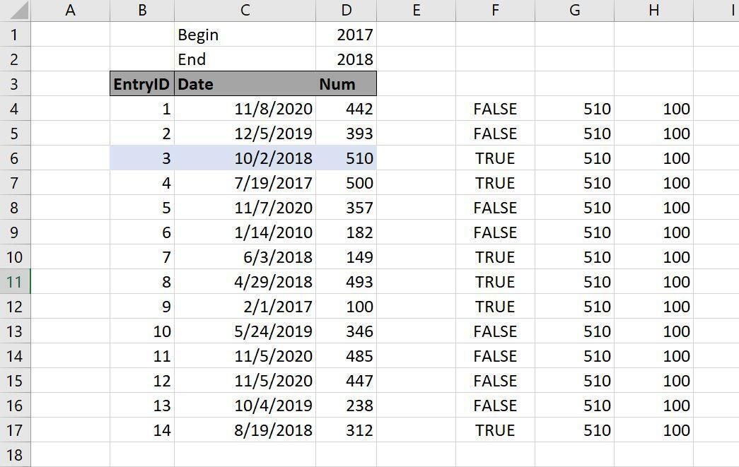
Figure F
If you enter a year that isn’t represented by a date value in column C, the rules continue to work. If neither date is represented, everything continues to work, but you might not realize why. Specifically, neither rule will be satisfied, so no record will be highlighted.